Exploratory Data Analysis • OSD758

Gene Expression

Let us start by loading the gene expression in long format, i.e. one row per gene × sample combination.

library(ggplot2)
library(dplyr)
library(OSD758)

(counts <- gene_expression())
#> # A tibble: 1,989,400 × 4
#>    sample_id           ensembl_gen_id     gene_symbol counts
#>    <chr>               <chr>              <chr>        <int>
#>  1 MHU-8_RTN_FLT_FLT02 ENSMUSG00000000001 Gnai3         2132
#>  2 MHU-8_RTN_FLT_FLT02 ENSMUSG00000000003 Pbsn             0
#>  3 MHU-8_RTN_FLT_FLT02 ENSMUSG00000000028 Cdc45          109
#>  4 MHU-8_RTN_FLT_FLT02 ENSMUSG00000000031 H19             29
#>  5 MHU-8_RTN_FLT_FLT02 ENSMUSG00000000037 Scml2           92
#>  6 MHU-8_RTN_FLT_FLT02 ENSMUSG00000000049 Apoh            22
#>  7 MHU-8_RTN_FLT_FLT02 ENSMUSG00000000056 Narf          3614
#>  8 MHU-8_RTN_FLT_FLT02 ENSMUSG00000000058 Cav2          3464
#>  9 MHU-8_RTN_FLT_FLT02 ENSMUSG00000000078 Klf6          2464
#> 10 MHU-8_RTN_FLT_FLT02 ENSMUSG00000000085 Scmh1         2779
#> # ℹ 1,989,390 more rows

Most expressed genes

Calculating median counts per gene:

median_gene_expression <-
  counts |>
  dplyr::group_by(ensembl_gen_id, gene_symbol) |>
  dplyr::summarise(median_counts = median(counts), .groups = "drop") |>
  dplyr::arrange(desc(median_counts))

median_gene_expression
#> # A tibble: 56,840 × 3
#>    ensembl_gen_id     gene_symbol median_counts
#>    <chr>              <chr>               <int>
#>  1 ENSMUSG00000030324 Rho               2727317
#>  2 ENSMUSG00000118841 Rn7s2             1778641
#>  3 ENSMUSG00002076161 Rn7sk             1516195
#>  4 ENSMUSG00000092837 Rpph1              901160
#>  5 ENSMUSG00000034837 Gnat1              773424
#>  6 ENSMUSG00000118866 Rn7s1              588929
#>  7 ENSMUSG00000041534 Rbp3               566448
#>  8 ENSMUSG00000092341 Malat1             553265
#>  9 ENSMUSG00000029064 Gnb1               537503
#> 10 ENSMUSG00000023978 Prph2              397989
#> # ℹ 56,830 more rows

The mostly expressed gene is rhodopsin (Rho) with a median of over 2.7 million reads, perhaps not so surprising given that these RNAseq samples are from retina.

Not expressed genes

On the contrary we have also genes that are not expressed at all. Actually, one-third of all genes (19,028) show no expression whatsoever in mouse retina:

total_gene_expression <-
  counts |>
  dplyr::group_by(ensembl_gen_id, gene_symbol) |>
  dplyr::summarise(total_counts = sum(counts), .groups = "drop") |>
  dplyr::arrange(desc(total_counts))

total_gene_expression |>
  dplyr::filter(total_counts == 0L)
#> # A tibble: 19,028 × 3
#>    ensembl_gen_id     gene_symbol total_counts
#>    <chr>              <chr>              <int>
#>  1 ENSMUSG00000000003 Pbsn                   0
#>  2 ENSMUSG00000000606 Vmn2r88                0
#>  3 ENSMUSG00000000690 Hoxb6                  0
#>  4 ENSMUSG00000000701 Tcl1b5                 0
#>  5 ENSMUSG00000000938 Hoxa10                 0
#>  6 ENSMUSG00000001168 Oas1h                  0
#>  7 ENSMUSG00000001656 Hoxc11                 0
#>  8 ENSMUSG00000001657 Hoxc8                  0
#>  9 ENSMUSG00000001819 Hoxd13                 0
#> 10 ENSMUSG00000001823 Hoxd12                 0
#> # ℹ 19,018 more rows

Gene expression distribution

The gene expression distribution is extremely skewed as one-third have no expression at all.

median_gene_expression |>
  ggplot(aes(x = median_counts)) +
  geom_density()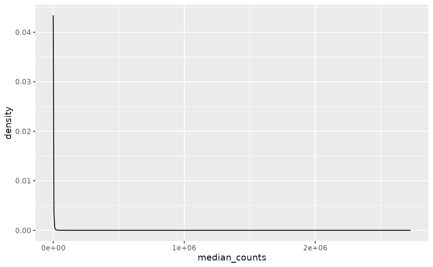

Removing genes with a median expression of zero counts still produces a very skewed distribution.

median_gene_expression |>
  dplyr::filter(median_counts != 0) |>
  ggplot(aes(x = median_counts)) +
  geom_density()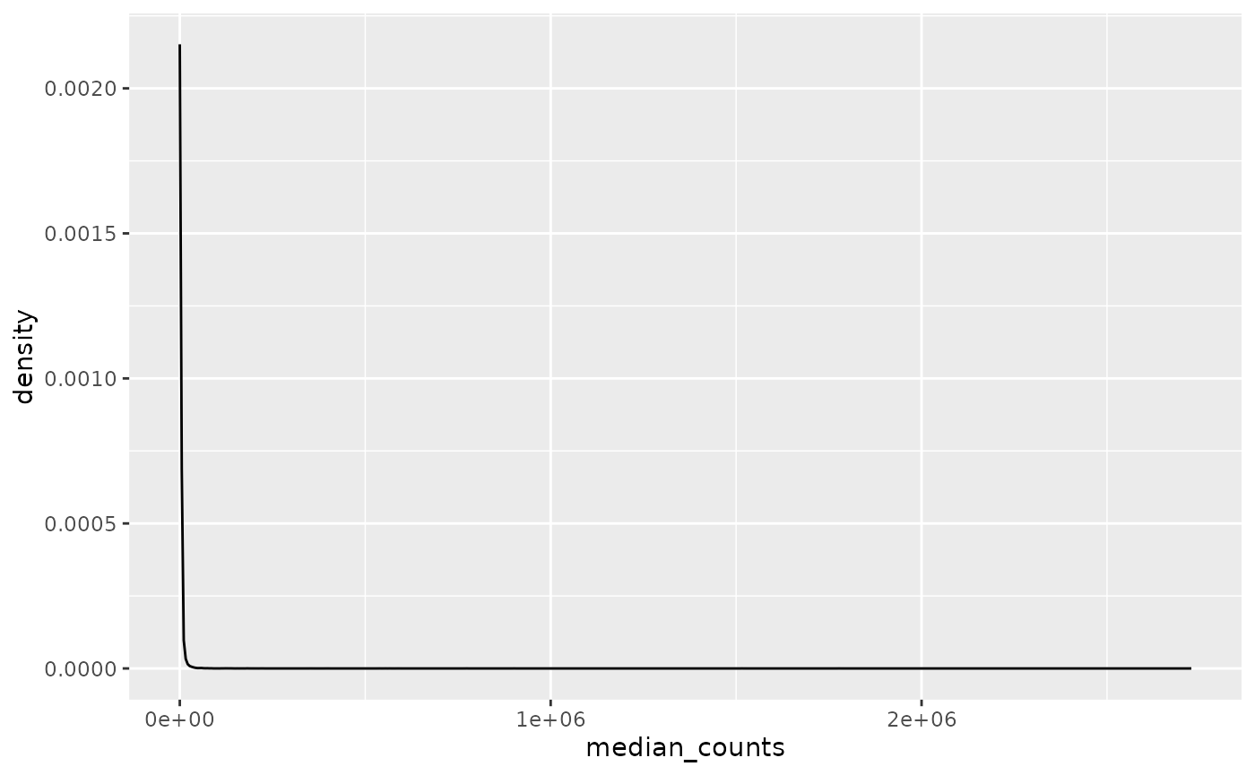

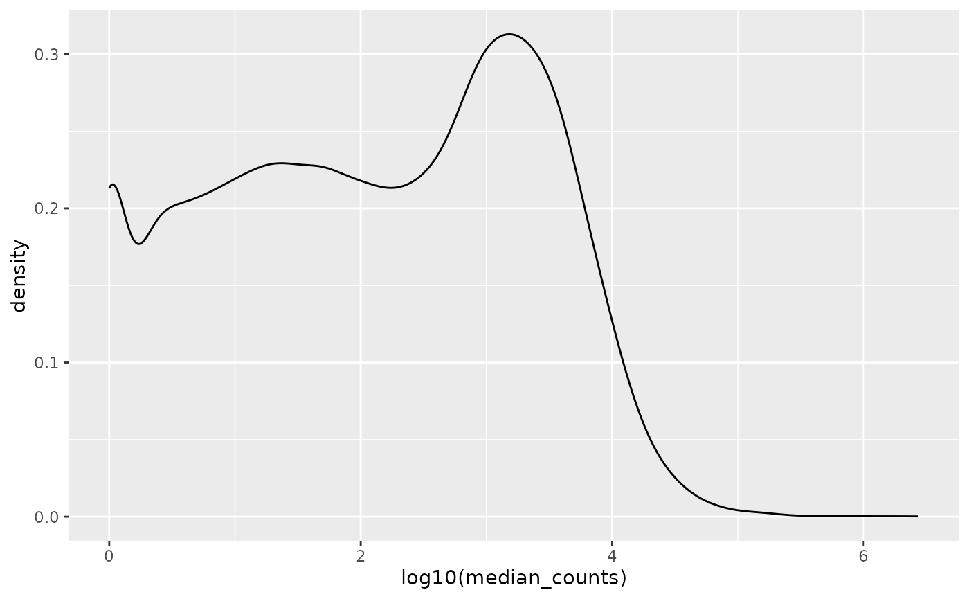
Log-scale transforming the median counts allows to conciliate very low counts with million count values, we can appreciate (roughly) three intervals:

Below 100 counts
Between 100 and 10,000 counts
Above 10,000 counts

median_gene_expression |>
  dplyr::filter(median_counts != 0) |>
  ggplot(aes(x = log10(median_counts))) +
  geom_density()